Tutorials
Eighteen short videos, one task each, recorded on the real interface. The first ten cover the basics. The other eight import an existing model and hand work to the agent.
English narration. Subtitles in English and Spanish.
The video plays from YouTube. Nothing loads from YouTube until you press play.
GWlink basics: MODFLOW 6 step by step
- 01 · 1:22
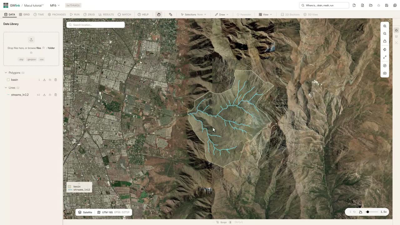
Load basin data into GWlink
Load a basin outline, stream lines and a terrain raster into the GWlink Data Library before building a grid. We use public sample data from Macul, near Santiago (UTM zone 19S), and check how the three files overlap in Layers.
- 02 · 1:16
Refine a Voronoi grid along streams
Build a Voronoi grid with 100 m base cells and 50 m cells along the streams, using a growth factor of 1.2 for a gradual transition. We also explain why these are target sizes, not identical cell widths.
- 03 · 1:25
Turn a stream shapefile into drain cells
Link the stream shapefile to the DRN package. The drain elevation uses the expression model top minus one, and conductance is an example value of 1000 m²/d. We also cover when to use a river package instead.
- 04 · 1:25
Change a pumping curve without changing stress periods
Edit one point of a named pumping curve, from -150 to -225 at day one, while the stress periods and time steps stay the same. Periods define the schedule. Curves define the values over time.
- 05 · 1:21
Run MODFLOW 6 and check the water budget
Validate the model, write the input files, run the solver and check convergence. Then open ZBUD to compare total inflow and outflow and read the discrepancy.
- 06 · 1:18
Read simulated heads in plan view
A head map needs a variable, a layer, a time and a scale. We attach a head file, switch layers and times, read the colour scale and draw contours every 0.5 m.
- 07 · 0:59
Groundwater heads in 3D: top view and iso surfaces
Colour a ten-layer model by head in the 3D viewer, look at it from above, then turn on surfaces of equal head and turn the model to see them cross the layers.
- 08 · 1:55
Backward particle tracking with PRT
Where could water at this point have come from? Load a release point from a CSV, add the PRT package with backward tracking and effective porosity, run the flow model and then PRT from RUN. Read the travel time and why the path stopped, in plan and 3D.
- 09 · 1:12
Read your model as a FloPy notebook
GWlink generates a Python notebook from the current model. We find the recharge package in the FloPy code and check that it uses the same value shown in the GUI.
- 10 · 1:31
Watch a solute plume grow over time
Add the transport package to a completed flow run, set the well concentration to 1000 mg/L in PACKAGES and run it once from RUN. On a fixed logarithmic colour scale, move the output time from day 1 to day 366 and watch the plume grow downstream. Uses the flow model of MT3DMS problem 3.
GWlink: import and the agent
- 11 · 1:55
Ask the GWlink agent to change recharge
Ask the agent to halve recharge and run the model, then check the saved value and the new run's convergence yourself. The chat explains the work. The model and the run confirm it.
- 12 · 1:41
Import an existing MODFLOW 6 model
Point GWlink at a folder with mfsim.nam, import it into its own workspace and read the import report and package badges. Then validate, write and run the imported copy.
- 13 · 1:28
Ask the agent to build a Voronoi grid
Starting from a loaded basin with no cells, ask the agent for a Voronoi grid with 100 m target cells. Then check the boundary, target size and cell count in GRID.
- 14 · 1:37
Ask the agent to refine an existing grid
Save a grid snapshot, then ask for 50 m cells along the streams while keeping the 100 m base. Compare the old and new meshes and their cell counts.
- 15 · 1:55
Ask the agent to add drains along a stream
One request links the stream line to a DRN source with elevation at model top minus one and conductance of 1000 m²/d. Then inspect the saved source and the affected cells in Packages.
- 16 · 2:06
Ten stress periods, one request to the agent
Double the length of ten stress periods that range from 5 to 14 days, while keeping the other time settings. Then check every row in TIME.
- 17 · 2:42
Teach the agent once, then replay the change
Save the agent's accepted actions as a named flow, return to the original project, validate the flow and replay it.
- 18 · 1:08
Milford in 3D: heads, iso surfaces and satellite terrain
Show the Milford model's heads in 3D, add surfaces of equal head, then add the land surface with the satellite image draped on it and turn the view to read the valley.
To follow the tutorials on your own data, request access.
GWlink is in private beta, by invitation.